What I have learnt from dogs and cats

Motivation

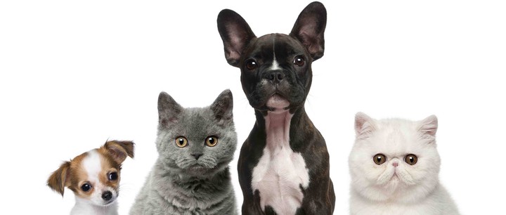
To specialize further in image classification I decided to try a classic challenge in this area: the Kaggle competition Dogs vs Cats. By taking part in the challenge we can easily use their data set (25k labeled images) and 12.5k unlabeled test images. Each sample from the data set is a varied-sized RGB image containing either a dog or a cat and our task is to decide to which class the sample belongs. We can also compare our results to other users and have some indicatives of where our model could improve.

In particular, in this post I would like to address the following topics: transfer learning, the effects of the input image size and regularization on the model performance.

Transfer learning approach

Transfer learning is the technique of using previously trained models for a specific purpose on a different problem. This can be done by tuning the model parameters on the new problem data set. It is advantageous because the trained model might have valuable feature-extraction capabilities that can be useful if the application domain of the two problems are similar (i.e., object classification). So instead of training the whole model from scratch we just fine-tune the few last layers (responsible for the classification) to the new problem data set.

Before designing my own architecture I considered fine-tuning good performing models on hard challenges such as the ImageNet Large Scale Visual Recognition Challenge (ILSVRC). One of these models is the winner of the ILSVRC 2014 Classification+localization challenge, VGG-16 model, organized in 5 convolutional blocks and a dense block. The convolutional blocks group 2-3 convolutional layers in sequence with a max-pooling layer to reduce dimensionality. In total there are 13 convolutional layers and 3 dense layers. The original challenge data set had 1000 classes so the output layer has 1000 output units.

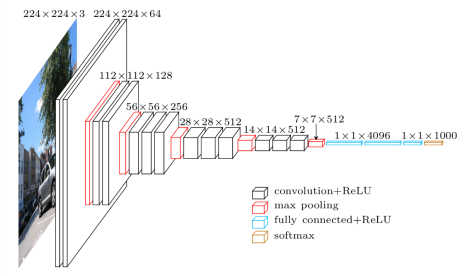
Since we are only dealing with two classes we must adapt the architecture by replacing the three dense layers with a single dense layer containing two softmax activation units. It is reasonable to replace the three layers with a single one because the model has enough complexity, so the features at this point (~ 25k of them) are already high level ones, which can easily determine the image class without further layers.

To fine tune the model parameters to dogs-vs-cats classification we assume the 13 conv-layers provide good enough features, so we freeze their parameters and allow only the last layer parameters to be updated. This model has a large number of parameters: the 13 conv-layers provide 14,714,688 parameters while the final dense layer has 50,178 parameters. Clearly it is much simpler to fit just these final layer parameters instead of the whole network, which allows us to use our modest data set on this structure.

The original model image input size was 224 x 224, and although this changes the dimension of the following convolutional layers, their filter sizes are kept the same, so we can still use the weights from the original model, except for the final dense layers, where the weights depend upon the number of units in each layer. Since we replaced the final dense layers we could have chosen any given input size. To keep the original design we kept the standard input dimension. Another consideration is that the pre-processing should be the same assumed by the VGG model, that is, the pixel intensities are not normalized and are kept in the original range $[0,255]$.

In order to evaluate the model we split the labeled samples into 20k training samples and 5k test samples, since the 12.5k samples provided for evaluation are not labeled. After 10 training epochs we achieved great performance on both the training and test set, as seen on the learning curve below. You can check the notebook with this experiment here.

Analyzing the results we clearly see that the model performs very well both on training and test sets with accuracy higher than 95% on the test set. This performance can be explained by the complexity of the model and the amount of information it has been trained upon. Even though it performs well and was quite simple to implement, it is a rather heavy model with ~14 million parameters. This leads to the question of whether we can get a similar performance using a simpler, more computational efficient model.

Custom model architecture: dognet

Since the VGG model was successful in the previous attempt, it is worth considering its architecture as base to a simpler custom model called dognet. Similarly, we organize the convolutional blocks with two conv layers followed by a max-pooling layer, and a final single filter conv layer to merge all feature maps into one. So the new model architecture will have 7 convolutional layers, all using 3x3 filters and RELU activation, with decreasing number of filters: 32, 32, 16, 16, 4, 4, 1. After flattening the last conv layer, a dense layer with 2 outputs and softmax activation is used as the network output, interpreted as class probabilities.

A important difference in this model is that we insert a batch normalization layer after the input layer with the purpose of normalizing the input across the entire batch, which leads to faster convergence and improved training. Note that the input images pixels values are also scaled into the range of $[0,1]$ by multiplying all the channels by $\frac{1}{255}.$

The proposed model uses 18,829 parameters, less than 1% of the amount of VGG parameters. We still assume the input image size as 224x224. The first experiment was to check the model had enough capacity to fit the data, meaning it would not underfit the data. So we trained using Adadelta optimizer with no regularization for about 100 epochs. We were able to obtain 100% accuracy on the training set, which proves the model had enough capacity for the data. The performance on the test set, however, was not so satisfactory: 79% accuracy. This suggests a strong overfitting, which is expected as no regularization was used.

Size matters?

An issue faced during the first experiment was the time required to train the model: using only an i5 CPU (4 cores) each epoch took about 40 minutes, so training for a 100 epochs took a few almost three days. To reduce training time the images were resized to 64x64 pixels, which had astonishing effects on the temporal performance: an epoch took only 200s to train. This input downscaling did not impact the amount of model parameters so much: there are now 17,869, opposed to the early 18,829 parameters. This is reasonable since most of the network is convolutional, so the number of parameters will not change with the input size, just on the dense layers, which happens to be the case of the final one. In this case very few parameters depend on the input size.

This downscaled input model, with 100 epochs of training, achieved 98% accuracy on the training set and 80% accuracy on the test set, so still overfitting. This performance is very similar to the one observed on the original input size (224x224), which leads to thinking that in this case downscaling the input is a good choice since it allows faster training times without affecting the model performance.

Regularization

Previous training attempts resulted in model overfitting, which happens when the model performs well on the training set but poorly on the test set. It is generally caused because the model capacity is greater than the volume of data available for training, thus causing the model to specialize on fine characteristics (noise) specific to the training data and prevent the generalization expected in the test set. To overcome this problem regularization techniques must be employed to balance the model capacity and the amount available data, enforcing that simpler, more general models are obtained.

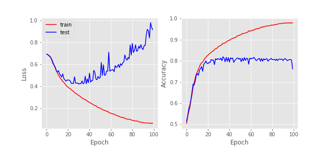
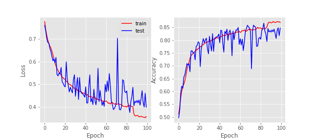
In order to observe this effect in more detail we can observe the following figure, showing the progression of the model loss and accuracy as the training process evolve. It is clear that overfitting becomes pronounced around epoch 20, and the test accuracy becomes steady at 80% from this point forward.

L2 norm

Firstly, L2-norm regularization is applied. This method adds a regularization term on the loss function corresponding to the L2-norm metric of a layer weights, penalizing large parameters of the network, as shows the next equation, where $L_t(w)$ is the loss correspondent to training errors (in this case log-loss).

$$ L(w) = L_t(w) + \lambda \Vert w \Vert^2 $$

This means the model is looking for finding parameters that both result in low training error, but are also small, which means simpler models and more generalization. This trade-off is tuned through the hyper-parameter $\lambda$, with higher values prioritizing model simplification. The L2 specific effect is introducing a negative parcel to the parameters updates (coming from the gradient of the regularization term), so the weights tend to become smaller at each iteration.

By applying this technique with moderate regularization $\lambda=10^{-3}$ on all layers, we obtained the following progression of model loss and accuracy. A note aside is that the model should be randomly initialized for training, if the previous weights (obtained without regularization) are used for initialization the model will not be able to improve generalization.

The model still overfits, but observe that the test set accuracy has actually improved, now becoming steady at 85%, showing that regularization has improved the model generalization on new samples.

We could try a stronger regularization with $\lambda=10^{-2}$, but perhaps we could enhance regularization by aggregating a different technique called dropout.

Dropout

Dropout works by deactivating a set of random units of a given layer during training phase. Such practice have a good impact on the network because it removes inter-layer co-adaptation, thus avoiding any unit to rely too much on a single previous unit, so enabling generalization. The strength of the regularization is controlled by a hyper-parameter that represents the rate of the layer units to drop. It is commonly applied before dense layers, but could also be used for convolutional ones.

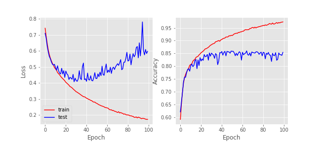
Combining both L2-norm with $\lambda=10^{-3}$ on all layers and dropout regularization with ratio 0.5 (half units dropped) on convolutional layers, we obtain the following loss and accuracy:

The results show that combining L2 and dropout regularization provides a good solution to prevent model overfitting. Even though the model did not overfit we did not observe any improvement on the test set accuracy if compared to L2 only regularization. Another interesting characteristic is the chaotic behavior of the test loss function, which is due to the probabilistic nature of the unit drops, albeit the mean value of the test loss seems to follow the train loss, which is a good indicative. The notebook containing the dognet architecture along with regularizers is available here.

Conclusion

In this specific application the downscaling of input image size did not have a bad impact on model performance and was actually capable of greatly decreasing the training time. Although this may not be the case when dealing with samples containing fine details where two distinct classes look similar to one another.

Through the series of experiments applying regularization techniques it was possible to prevent model overfiting and improve generalization measured as an increase on test set accuracy, getting up to 85% accuracy. Combining both L2 and dropout proved to be a good idea.

In order to further increase model accuracy on the test set it would be necessary to gather more training data and possibly apply data augmentation (rotation, scaling, cropping). Another possibility is to use the transfer learning approach, which uses already trained high-level models, offering higher than 96% accuracy on the test set, at the expense of having a much larger model and longer processing times.

Finally, a note on the Kaggle competition. I think Kaggle has an important role on promoting machine learning and its applications, in engaging researchers and hobbyists alike and even helping people to learn more about recent techniques, letting them compare results, etc. Still, it seems to fail to consider the complexity of the elaborated solutions. To illustrate my point check the Marco Lugo post on Kaggle blog showing his 3rd place solution to this challenge. He uses a bunch of complex convolutional models in parallel and predict the output as a weighted average of these classifiers. Of course great results come at the price of increased complexity. I am just saying that complexity should also be taken in account when evaluating model. We may ask ourselves: what is the best score I can get using only the training data they provide, without any pre-loaded models, or an ensemble of 20 complex classifiers? The way Kaggle is organized today does not allow an answer to that question.